How to solve ODE in OpenFOAM

Mathematical background

In order to solve any high order ODE numerically, it should be reduced first to a system of first order ODEs. This process of order reduction produces a number of ODEs equal to the order of the original ODE. Here, the reduction process as described by Ferziger [2] for general high order ODE,

\begin{equation*} y^n = f(x,y,y',\cdots y^{n-1}) \end{equation*}

where \(n\) is the order. Then it can be redefined as (transformation),

\begin{align*} y_1 &= y \\ y_j &= y^{j-1} \quad j=1,2,\cdots n-1 \end{align*}

Finally, the system could be represented as (differentiation),

\begin{align*} f_j = y'_j &= y_{j+1} \quad j=1,2,\cdots n-1\\ f_n = y'_n &= f(x,y_1,y_2,\cdots y_n) \end{align*}

As described above, the process could be summarised into two steps; a transformation of variables and differentiation. In OpenFOAM, there is an extra step required for stiff system solvers only. These solvers require the jacobian matrix and the time partial derivatives.

\begin{equation*} J = \begin{bmatrix} \frac{\partial f_1}{\partial y_1} & \frac{\partial f_1}{\partial y_2} & \cdots &\frac{\partial f_1}{\partial y_n}\\ \frac{\partial f_2}{\partial y_1} & \frac{\partial f_2}{\partial y_2} & \cdots &\frac{\partial f_2}{\partial y_n}\\ \vdots & \vdots & \ddots & \vdots \\ \frac{\partial f_n}{\partial y_1} & \cdots & \cdots &\frac{\partial f_n}{\partial y_n} \end{bmatrix} \end{equation*}

Where \(f_n\) is the equation \(n\) in the reduced system. Also the partial derivative with respect to \(x\) (independent variable)

\begin{equation*} \frac{\partial f_1}{\partial x} \cdots \frac{\partial f_n}{\partial x} \end{equation*}

Equation of motion

The equation of motion of single degree of freedom system (simple mass-spring system) , which is a second order ODE, will be used here as an example.

\begin{align*} m\ddot{q} + kq &= 0 \\ \ddot{q} &= -\frac{k}{m}q \end{align*}

where \(m\) is the mass, \(k\) is the stiffness and \(q\) is the displacement.

This equation has an exact solution represents the harmonic oscillation of the system as (assuming zero initial velocity);

\begin{equation*} q = q_0 \cos(\omega t) \end{equation*}

where \(q_0\) is the initial displacement and \(\omega\) is the natural frequency of the system \(\omega=\sqrt{k/m}\).

It is the time to apply the methodology described in the previous section (Mathematical background) on the equation of motion.

• Step A: Transformation from \(q\) to \(y\)

  \begin{align*} y_1 &= q \\ y_2 &= \dot{q} \end{align*}

• Step B: Differentiation (substitute first)

  \begin{equation*} \ddot{q} = -\frac{k}{m}y_1 \end{equation*}

  then,

  \begin{align*} f_1 = \dot{y_1} &= \dot{q} \\ &= y_2\\ f_2 = \dot{y_2} &= \ddot{q} \\ &= -\frac{k}{m}y_1 \end{align*}

• Step C: Jacobian (optional)

  The Jacobian matrix is required for stiff solvers only. For this case, it is just \((2\times2)\) matrix,

  \begin{equation*} J = \begin{bmatrix} 0.0 & 1.0 \\ -k/m & 0 \end{bmatrix} \end{equation*}

  and time derivatives (independent variable in this case),

  \begin{align*} \frac{\partial f_1}{\partial t} &= 0 \\ \frac{\partial f_2}{\partial t} &= 0 \end{align*}

Where to start?

It is typical in OpenFOAM to search for a similar implementation as a starting point. Fortunately, there is a small test program included in OpenFOAM source files. It is described in details in [3]. So copy it to your run directory then compile and run it. (RKCK45 is one of OpenFOAM ODE solvers).

$ cp -r $FOAM_APP/test/ODE .
$ wmake
$ Test-ODE RKCK45

You should get a lot of numbers on the screen and finally you should see;

Analytical: y(2.0) = 4(0.223891 0.576725 0.352834 0.128943)
Numerical:  y(2.0) = 4(0.223891 0.576725 0.352835 0.128943), dxEst = 0.402302

Please note that since OpenFOAM-2.3 version, the ordinary differential equation solvers have been updated [4]. Therefore Zongyuan [3] report has some outdated parts.

Implementation

The reduction step is essential to solve the equation and as it is described above. This step is important in OpenFOAM and in any other code like python or Octave/Matlab. The implementation in OpenFOAM is divided into two main classes; ODEsystem and ODEsolver. From its name you can guess the function of each class. ODEsystem is an abstract class defines the system of first order ODEs as explained above. ODEsolver is the base class for all the ODE solvers in OpenFOAM.

Back to Test-ODE.C, open it in any text editor (I prefer atom or qt-creator for big projects) and start examining the code. You will notice that the code is divided into two parts, the first part is the definitionn of class called testODE and the second part is the main function.

class myODE
:
public ODESystem
{
    //- Mass of the system
    const scalar m_;
    //- Stiffness of the system
    const scalar k_;

    public:

    myODE(const scalar& mass, const scalar& stiffness)
    :
    ODESystem(),
    m_(mass),
    k_(stiffness)
{}

label nEqns() const
{
    return 2;
}

void derivatives
(
    const scalar x,
    const scalarField& y,
    scalarField& dydx
) const
{
    dydx[0] = y[1];
    dydx[1] = -(k_/m_+VSMALL)*y[0]
}

void jacobian
(
    const scalar x,
    const scalarField& y,
    scalarField& dfdx,
    scalarSquareMatrix& dfdy
) const
{
    dfdx[0] = 0.0;
    dfdx[1] = 0.0;

    dfdy[0][0] = 0.0;
    dfdy[0][1] = 1.0;

    dfdy[1][0] = -(k_/m_+VSMALL);
    dfdy[1][1] = 0;
}

 1
 2
 3
 4
 5
 6
 7
 8
 9
10
11
12
13
14
15
16
17
18
19
20
21
22
23
24
25
26
27
28
29
30
31
32
33
34
35
36
37
38
39
40
41
42
43
44
45
46
47
48
49
50
51
52
53
54

int main(int argc, char *argv[])
{
    argList::validArgs.append("ODESolver");
    argList args(argc, argv);

    // system properties (mass and stiffness)
    const scalar mass = 2.0; // Kg
    const scalar stiff = 2048.0; // N/m
    // Initial displacement
    const scalar y0 = 0.2; // m
    const label n = 200;
    const scalar endTime = 1.0; // s

    // Create the ODE system as object of type myODE
    myODE ode(mass,stiff);

    // Create dictionary and add the odeSolver name
    dictionary dict;
    dict.add("solver", args[1]);

    // Create the selected ODE system solver
    autoPtr<ODESolver> odeSolver = ODESolver::New(ode, dict);

    // Initialise the ODE system fields

    // Start time
    scalar xStart = 0.0;
    // time step
    const scalar dx = endTime/n;
    // Initial displacement and velocity
    scalarField yStart(ode.nEqns());
    yStart[0] = y0;
    yStart[1] = 0.0;
    // integration initial step
    scalar dxEst = 0.1;
    scalar xEnd = 0;

    // Required to store dydx
    scalarField dyStart(ode.nEqns());

    // Integration loop
    for (label i=0; i<n; i++)
    {
        xEnd = xStart + dx;
        ode.derivatives(xStart, yStart, dyStart);
        odeSolver->solve(xStart, xEnd, yStart, dxEst);
        xStart = xEnd;
        Info << xStart << "   " << yStart[0] << endl;
    }

    Info<< "\nEnd\n" << endl;

    return 0;
}

$ wmake
$ Test-ODE RKCK45 > log

Validation

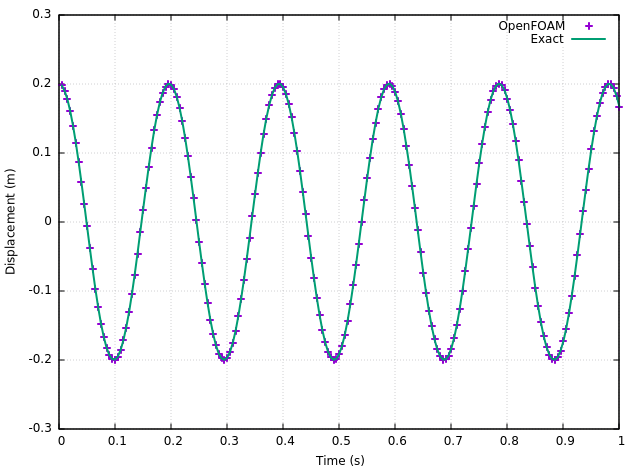
As mentioned before (Equation of motion), this ODE has an exact solution. It is basically a harmonic oscillation which could be represented as (after applying the initial conditions and system properties),

\begin{equation*} q(t) = 0.2 \cos(32t) \end{equation*}

A quick and easy way to compare the results is by using gnuplot to visualise the results.

# system properties
mass = 2.0
stiff = 2048.0
x0 = 0.2

set grid
set samples 200
set xlabel 'Time (s)'
set ylabel 'Displacement (m)'
set yrange [-0.3:0.3]

f(x) = x0*cos(sqrt(stiff/mass)*x)
plot 'log' u 1:2 w p lw 2 t "OpenFOAM", f(x) w l lw 2 t "Exact"

Final remarks

This post is meant to be minimal as possible and to be focused on solving ODE. Therefore, there are many possibilities to improve the main program. The system properties can be read from the command line directly or , even better, all the inputs could be included in one dictionary (OpenFoam style). Also, the output result could be formatted in a better elegant way. Moreover, the results can be written to a file. Finally, the solve function is an overloaded function, so it can be used with different input argument.

Please feel free to comment below. Your feedback will be highly appreciated.

• Update: 23 June 2016, scalar type added to myODE constructor as pointed out by Mohamed Ouda
• Update: 28 June 2016, variables names are revised to be consistent and more clear according to Francisco Angel comments